In systemPipeR/systemPipeShiny: systemPipeShiny: An Interactive Framework for Workflow Management and Visualization
```{css, echo=FALSE, eval=TRUE}
pre code {
white-space: pre !important;
overflow-x: scroll !important;
word-break: keep-all !important;
word-wrap: initial !important;
}
body {
max-width: 2000px !important;
}
.main-container {
max-width: 1800px !important;
margin-left: auto;
margin-right: auto;
}
```r
options(width=80, max.print=1000)
knitr::opts_chunk$set(
    eval=as.logical(Sys.getenv("KNITR_EVAL", "TRUE")),
    cache=as.logical(Sys.getenv("KNITR_CACHE", "TRUE")),
    tidy.opts=list(width.cutoff=60),
    tidy=TRUE,
    eval = FALSE)
# shiny::tagList(rmarkdown::html_dependency_font_awesome())
suppressPackageStartupMessages(library(systemPipeShiny))
knitr::include_graphics(path = "../inst/app/www/img/logo.png")
Introduction
systemPipeShiny
(SPS) extends the widely used systemPipeR
(SPR) workflow
environment with a versatile graphical user interface provided by a Shiny
App. This allows non-R users, such as
experimentalists, to run many systemPipeR's workflow designs, control, and
visualization functionalities interactively without requiring knowledge of R.
Most importantly, SPS has been designed as a general purpose framework for
interacting with other R packages in an intuitive manner. Like most Shiny Apps,
SPS can be used on both local computers as well as centralized server-based
deployments that can be accessed remotely as a public web service for using
SPR's functionalities with community and/or private data. The framework can
integrate many core packages from the R/Bioconductor ecosystem. Examples of
SPS' current functionalities include: (a) interactive creation of experimental
designs and metadata using an easy to use tabular editor or file uploader; (b)
visualization of workflow topologies combined with auto-generation of R
Markdown preview for interactively designed workflows; (c) access to a wide
range of data processing routines; (d) and an extendable set of visualization
functionalities. Complex visual results can be managed on a 'Canvas Workbench'
allowing users to organize and to compare plots in an efficient manner combined
with a session snapshot feature to continue work at a later time. The present
suite of pre-configured visualization examples include different methods to
plot a count table. The modular design of
SPR makes it easy to design custom functions without any knowledge of Shiny,
as well as extending the environment in the future with contributions from
the community.
This vignette only includes the basics of SPS. For full documentations of SPS,
visit our website at: https://systempipe.org/sps.
Demos
SPS has provided a variety of options to change how it work. Here are some examples. At the time of writing, there is an interactive tutorial (guide) embedded in the demos
that users can access from the upper-right corner. The tutorial introduces
major functionalities of SPS.
| Type and link| option changed | notes |
| --- | --- | --- |
| Default full installation | See installation | full app, may take longer (~15s) to load |
| Minimum installation | See installation | no modules installed |
| Login enabled | login_screen = TRUE; login_theme = "empty" | no modules installed |
| Login and login themes | login_screen = TRUE; login_theme = "random" | no modules installed |
| App admin page | admin_page = TRUE | use the link or simply add "?admin" to the end of URL of any demos |
For the login required demos, the app account name is "user" password "user".
For the admin login, account name "admin", password "admin".
Please DO NOT delete or change password when you are trying the admin features.
Although shinyapps.io will reset the app once a while, this will affect other people
who are viewing the demo simultaneously.
Installation
Full
if (!requireNamespace("BiocManager", quietly=TRUE))
    install.packages("BiocManager")
BiocManager::install("systemPipeShiny", dependencies=TRUE)
This will install all required packages including suggested packages that
are required by the core modules. Be aware, it will take quite some time if you
are installing on Linux where only source installation is available. Windows and Mac
binary installations will be much faster.
Minimum
To install the package, please use the BiocManager::install command:
if (!requireNamespace("BiocManager", quietly=TRUE))
    install.packages("BiocManager")
BiocManager::install("systemPipeShiny")
By the minimum installation, all the 3 core modules are not installed. You
can still start the app, and when you start the app and click on these modules,
it will tell to enable these modules, what packages to install and waht
command you need to run.
Just follow the instructions. Install as you need.
Most recent
To obtain the most recent updates immediately, one can install it directly from
GitHub as follow:
if (!requireNamespace("remotes", quietly=TRUE))
    install.packages("remotes")
remotes::install("systemPipeR/systemPipeShiny", dependencies=TRUE)
Similarly, remotes::install("systemPipeR/systemPipeShiny") for the minimum develop
version.
Linux
If you are on Linux, you may also need the following libraries before installing SPS.
Different distributions
may have different commands, but the following commands are examples for Ubuntu:
sudo apt-get install -y libicu-dev
sudo apt-get install -y pandoc
sudo apt-get install -y zlib1g-dev
sudo apt-get install -y libcurl4-openssl-dev
sudo apt-get install -y libssl-dev
sudo apt-get install -y make
Main functionalities
Currently, SPS includes 5 main functional categories (Fig 1):
- Pre-defined modules include (open-box ready):
a. A workbench for designing and configuring data analysis workflows,
b. Downstream analysis and visualization tools for RNA-Seq, and
c. A space to make quick ggplots.
- A section with user custom tabs: users define their own SPS tabs.
- An image editing tab "Canvas" which allows users to edit plots made from
the previous two categories.
- Login / admin feature: deploy-ready app security and management toolkits.
- Deep customization: user defined app tabs, looking, notification, tutorials,
and more.
Besides, SPS provides many functions to extend the default Shiny development, like
more UI components, server functions and useful general R ulitlieslike error catching,
logging, and more. These functionalitlies are distributed as
SPS supporting packages: spsComps,
drawer, and spsUtil.

Figure 1. Design of systemPipeShiny.
The framework provides an
interactive web interface for workflow management and data visualization.
Within the functional categories, SPS functions are modularized in
sub-components, here referred to as SPS tabs that are similar to
menu tabs in other GUI applications that organize related and inter-connected
functionalies into groups. On the backend, SPS tabs are based on Shiny modules,
that are stored in separate files. This modular structure is highly extensible
and greatly simplifies the design of new SPS tabs by both users and/or developers.
Details about extending existing tabs and designing new ones are provided in
advanced sections on our website.
SPS example usage
The following instructions go through use each module step by step.
This vignette is the simplified version of instruactions. Due to package size limit,
we cannot write the full instructions here. We highly recommend you to read the full
details on our website: https://systempipe.org/sps/ for instructions,
animations, videos, and advanced sections.
Load package
Load the systemPipeShiny package in your R session.
library(systemPipeShiny)
Initialize SPS project
Before launching the SPS application, a project environment needs to be created with the
following command.
spsInit()
For this toy example, the project directory structure is written to a temporary
directory on a user's system. For a real project, it should be written to a
defined and user controlled location on a system rather than a temporary
directory.
sps_tmp_dir <- tempdir()
spsInit(app_path = sps_tmp_dir, change_wd = FALSE, project_name = "SPSProject")
sps_dir <- file.path(sps_tmp_dir, "SPSProject")
SPS project structure
The file and directory structure of an SPS project is organized as follows.
SPS_xx/
├── server.R               |
├── global.R               | Most important server, UI and global files, unless special needs, `global.R` is the only file you need to edit manually
├── ui.R                   |
├── deploy.R               | Deploy helper file
├── config                 | Important app config files. Do not edit them if you don't know
│   ├── sps.db             | SPS database
│   ├── sps_options.yaml   | SPS default option list
│   └── tabs.csv           | SPS tab information
├── data                   | App example data files
│   ├── xx.csv
├── R                      | All SPS additional tab files and helper R function files
│   ├── tab_xx.R
├── README.md
├── results                | Not in use for this current version, you can store some data been generated from the app
│   └── README.md
└── www                    | Internet resources
    ├── about              | About tab information
    │   └── xx.md
    ├── css                | CSS files
    │   └── sps.css
    ├── img                | App image resources
    │   └── xx.png
    ├── js                 | Javascripts
    │   └── xx.js
    ├── loading_themes     | Loading screen files
    │   └── xx.html
    └── plot_list          | Image files for plot gallery
        └── plot_xx.jpg
Launch SPS
By default, the working directory will be set inside the project folder automatically.
To launch the SPS Shiny application, one only needs to execute the following command.
shiny::runApp()
After the SPS app has been launched, clicking the "Continue to app" button
on the welcome screen will open the main dashboard (Fig.2).

Figure 2: Snapshot of SPS' UI.
- Welcome screen.
- Module tabs.
- User defined custom tabs.
- The Canvas tab.
- All SPS tabs has this description on top. It is highly recommend to click here
to expand and read the full the description for the first time.
Alternatively, when using RStudio one can click the 
Run App button in the top right corner.
In addition, in Rstudio the global.R file will be automatically
opened when the SPS project is created. Custom changes can be made inside this file
before the app launches. The advanced section explains how
to change and create new custom tabs.
Workflow management
The workflow management module in SPS allows one to modify or create the
configuration files required for running data analysis workflows in
systemPipeR (SPR). This includes
three types of important files: a sample metadata (targets) file, a
workflow file (in R Markdown format) defining the workflow steps, and workflow running
files in Common Workflow Language (CWL) format. In SPS, one can easily create
these files under the "Workflow Management" module, located in navigation bar
on the left of the dashboard (Fig2 - 2).
The current version of SPS allows to:
- create a workflow environment;
- create and/or check the format of targets / workflow / CWL files;
- download the prepared workflow files to run elsewhere, like a cluster;
- directly execute the workflow from SPS.
1. setup a workflow
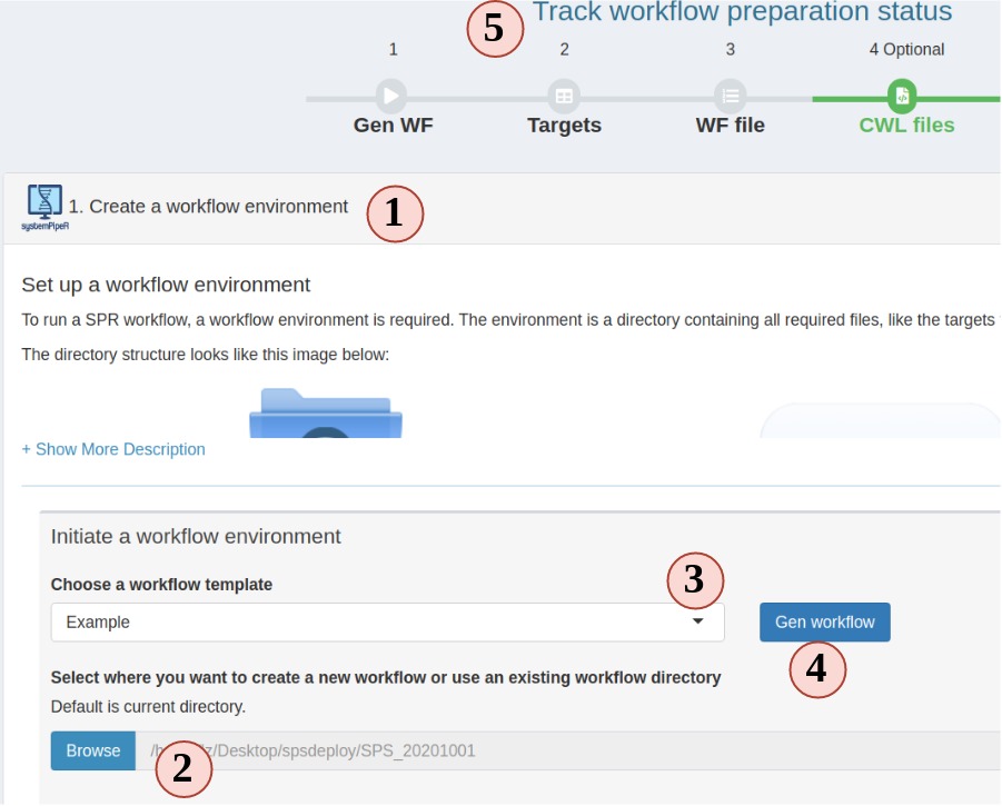
Figure 3. A. Workflow Management - Targets File
- In the workflow module, read the instructions and choose step 1. Step 1 should be
automatically opened for you on start.
- Choose a folder where you want to create the workflow environment.
- Choose a workflow template. These are SPR workflows and mainly are next-generation
sequencing workflows.
- Click "Gen workflow" to create the workflow project.
- You should see a pop-up saying about the project path and other information.
Clicking the pop-up will jump you to the step 2. The status tracker and banner for
step 1 should all turn green.
2. Prepare a target file
The targets file defines all input file paths and other sample information of
analysis workflows. To better undertand the structure of this file, one can
consult the "Structure of targets
file"
section in the SPR vignette. Essentially, this is the tabular file representation
of the colData slot in an SummarizedExperiment object which stores sample
IDs and other meta information.
The following step-by-step instructions explain how to create and/or modify targets
files using RNA-Seq as an example (Fig.3 A):
- Your project targets file is loaded for you, but you can choose to upload a different one.
- You can edit, right click to add/remove rows/columns (The first row is treated as column names).
- SPR target file includes a header block, that can also be edited in the SPS app. Each headers needs to start with a "#". Header is only useful for RNA-Seq workflow in current SPR. You can define sample comparison groups
here. Leave it as default for other projects.
- The section on the left provides sample statistics and information whether files exist inside the workflow project's
data directory. Choose any column you want from the dropdown to check and watch the statistics bar change in this section.
- statistic status bar.
- Clicking on "Add to task" can help you to check if your target file has any formatting problem. You should see a green success pop-up if everything is right. Now your target file is ready and you can click "save" to download it and later use in a SPR project.
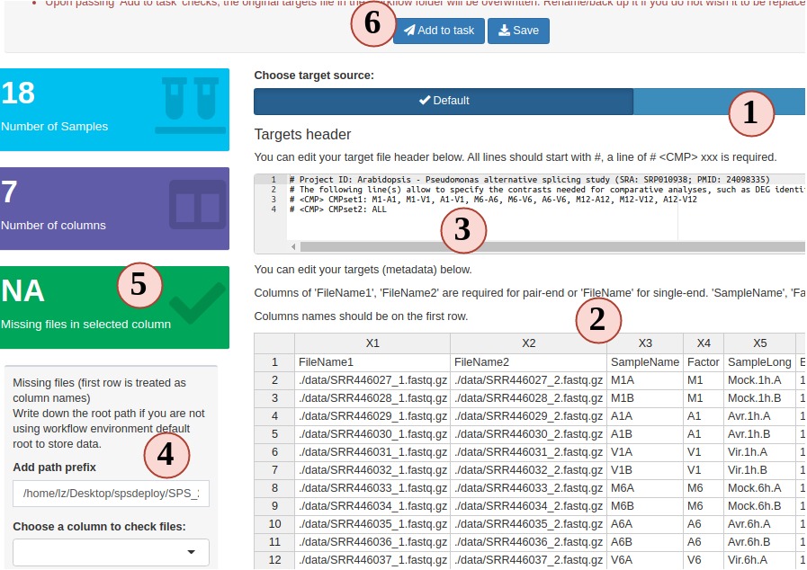
Figure 3. A. Workflow Management - Targets File
3. Prepare a workflow object
In SPR, workflows are defined in Rmarkdown files, you can read details and obtain them here.
Now let us follow the order below to see how SPS helps you to prepare a workflow file for a RNAseq project (Fig.3 B):
- The left panal is the workflow designer. All steps from the template from your
choosen workflow will be displayed here. The arrows indicates the execution order
of the entire workflow.
- All the steps are draggable. Drag and place steps to a different place to change the
order. Note: if you change the order, it may break the dependency. SPS will check
this for you. After changing orders, steps marked in pink mean these steps are
broken. You need to fix the dependency before you can save it.
- To config a step, such as, changing name, fixing dependency. Click the
button next to each step, a modal will show up and you can make changes there.
- To add a step, click the button. There, you will have
more options to choose which will be explained in the next figure.
- History is enabled in this designer, you can undo
or redo anytime you want.
Current SPS stores max 100 steps of history for you.
- To delete a step, simply drag it to the trash can.
- After you are done with all edits, click here to save the workflow so we can
run or download it in the next major step.
- On the right side is the workflow dependency plot. This plot shows how each
step is connected and the expected execution order. It does not mean the
the workflow will be run in the same order. The order is determined by the order
you have in the left-side designer.
- Enlarge the left or right panel. If you have a small monitor screen, this can help.

Figure 3. B.1 Workflow Management - Workflow Designer
R step and sysArgs step
On the designer there are two types of workflow steps. One is R step, which only
has R code. Then it is the time to run these R steps, they will be run in the same
R session as the Shiny app and in a separate environment different than your global
environment. In other words, all R steps are in the same environment, they can communicate
with each other, meaning you can define a variable in one step and use it in other
R steps.
sysArgs steps, on the other hand, is different, as its name suggest, it will invoke
system commands (like bash) when run. Details of how to create these steps will be
discussed on Fig 3.B.5, Fig 3.B.6.
View and modify steps
Current SPS allows users to view some basic information of R steps like, step name,
select dependency(ies). Besides, users are welcome to change the R code they want
in the second sub-tab (Fig 3.B.2).
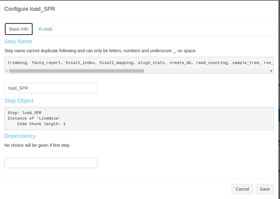
Figure 3. B.2 Workflow Management - config R
Modification of sysArgs steps is limited to step name and dependency. However, this
kind steps will provide more information to view, like the files that were used to
create this step, raw commandline code
that will be run, targets (metadata) and output dataframes. This information
is distributed in different subtabs (Fig 3.B.3).
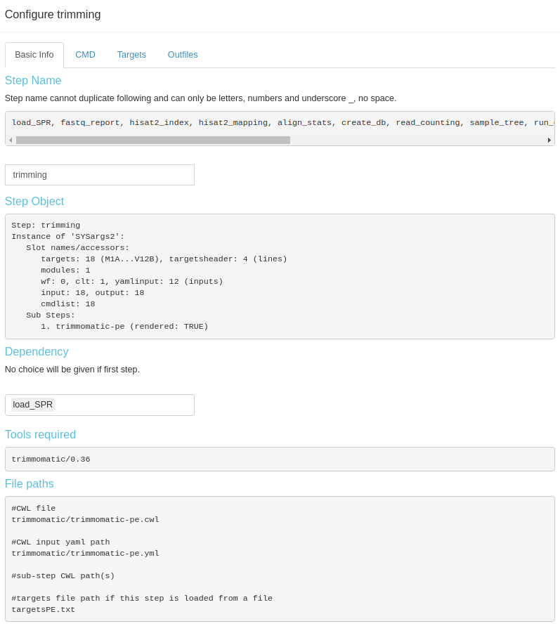
Figure 3. B.3 Workflow Management - config sysArgs
Create a new step
After clicking the button in Fig 3.B.1, you would need
to choose whether to create an R or sysArgs step (Figure 3. B.5).
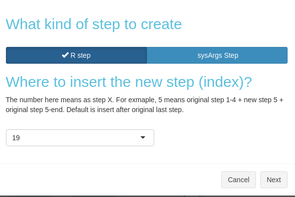
Figure 3. B.5 Workflow Management - Choose new step type
Create a new R step
Create a new R step is simple. In the modal, type the step name, R code,
and select dependency (Fig 3. B.6).
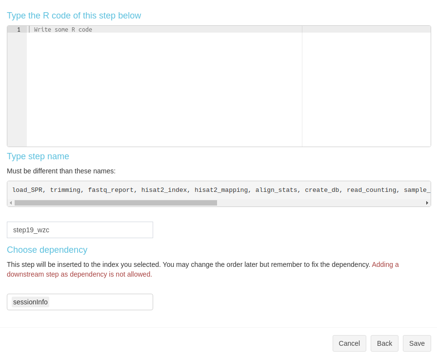
Figure 3. B.6 Workflow Management - New R step
Create a new sysArgs step
Basic info for sysArgs step is simialr to R step (Fig 3. B.7).
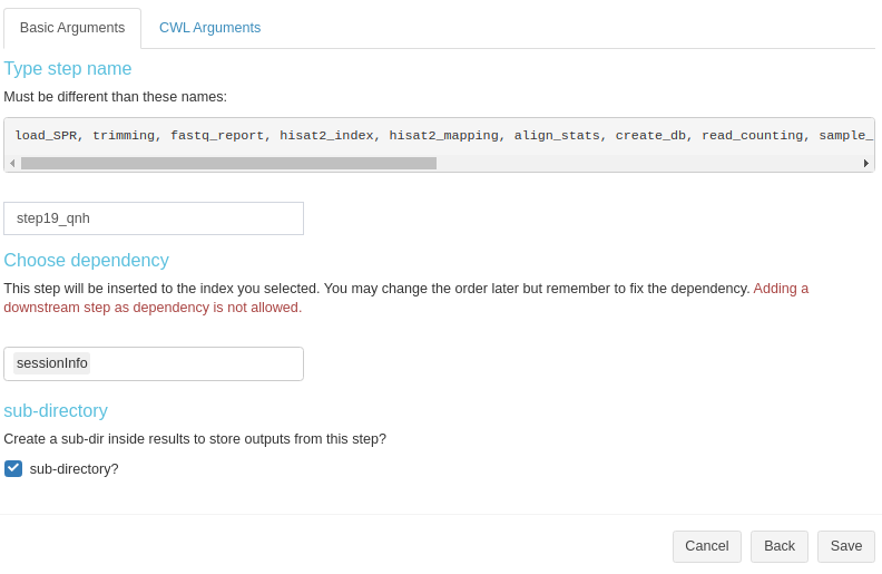
Figure 3. B.7 Workflow Management - New sysArgs step
To generate some commandline line, there are three items need to be prepared:
targets, CWL file, CWL yaml file (Fig.3. B.8).
- targets: metadata that will populate the basecommand sample-wisely. Columns in
targets will be injected into CWL yaml and then, yaml file will replace variables in parsed CWL base command.
- CWL file: provide the base command.
-
CWL yaml file: provides CWL variables.
-
Choose the targets source. Targets in SPR workflow steps can come from either a
fresh file or inherit from a previous sysArg step(s) (output from a previous
step can become input of the next(s)).
- If you choose from a previous step(s), select the steps from here. If a new
file, upload here.
- Then, the targets or inherited targets table is displayed here for you to take a
look. Later we will use these column to replace CWL yaml variables.
- Choose the CWL and CWL yaml file you want to use. All
.cwl and .yaml or .yml
files inside your workflow project param/cwl folder will be listed here. You
could drop more of these files you want to this folder. They will become aviable
the next time you create a new step.
- If you have all the three items, you can start to use which column from the targets
to replace each CWL yaml variables.
- Try to parse the command, see if the results is as what you expect. If not, try to
change options above and try again.
- If everything looks fine, save and create the step.
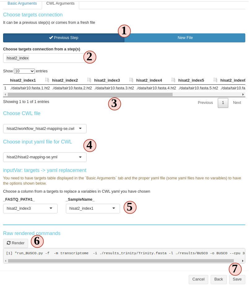
Figure 3. B.8 Workflow Management - New sysArgs step
4. Prepare CWL files (optional)
In the new version of SPR, all individual system workflow steps are called by the
CWL files. Each SPR workflow has a set of CWL files and normally users do not need
to make any change. In case you want to learn more about CWL and create some new
CWL files, Step 4 is a good place to practice.
To run a CWL step in SPR, 3 files are required:
- targets: to determine how many samples will be run and sample names.
- CWL running file: can be translated to bash code;
- CWL input: variables to inject into the running file
SPR is the parser between R and CWL by injecting sample information from targets
to CWL input file and then CWL parser translates it to bash code.
- Most people are not familiar this part, so read instructions carefully.
- Your project targets has been loaded for you, and an example CWL running and input
for hisat2 is also loaded for you. Directly parse the code. See what commandline
code you get.
- Change the targets injecting column, and parse again, see what has changed.
- You can edit the CWL running and input files
- Try to parse the new file and see what has changed.
- If new CWL files has been created, you can edit workflow Rmd files by adding your
new steps.
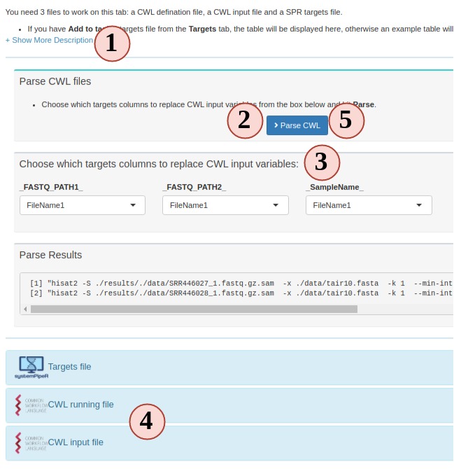
Figure 3. C. Workflow Management - CWL File
5. Run or finish workflow preparation
Up until this step, congratulations, the workflow is prepared. You can choose to
download the workflow project files as a bundle or continue to run the workflow.
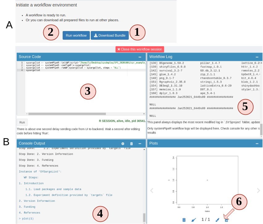
Figure 4.A.B Workflow Runner
- On step 5 you can choose to download the prepared workflow or directly run the
workflow. However, if you do not have the required commandline tools, workflow will
most likely fail. Make sure you system has these tools (Read about these tools).
- Open up the runner. It is a "Rstudio-like" interface.
- Code editor. Required workflow running code is pre-entered for you. You can simply
hit "Run" to start. Of course, you can delete the default code and run random R
code.
- Output R console.
- Workflow running log.
- View any plot output. and send a copy of your current plot to SPS Canvas tab or
download it.
RNA-Seq Module
This is a module which takes a raw count table to do normalization,
Differential gene expression (DEG) analysis, and finally helps users to generate
different plots to visualize the results.
Prepare metadata and count table
To start, we require two files, the metadata file (targets) and a raw count table (Fig. 5).

Figure 5 RNAseq
- This is the RNAseq module UI when you first click it. All sub-tabs are disbled
at the beginning. Other tabs will enabled as you proceed with different options.
- First, we need a metadata file to tell SPS what samples and conditions to use.
Here, we use the metadata file from SPR, which is also known as "targets" file.
If you are not familiar with the targets file, we suggest to use the workflow module
step 2 to practice creating and checking the format. You can also use the example to
see how it looks like.
- The loaded targets table is display here. You can use the box below each column
name to filter what samples to include/exclude. Only the "SampleName" and "Factor"
columns are used, other columns are ignored.
SampleName should be a unique character
string without space for each row. Factor is the experiment design factors, or
conditions, or treatments.
- If you want to DEG analysis, DEG comparison groups are defined in the targets
file header.
- The header will be parsed into comparison groups which contain individual comparisons.
If the parsed comparison is not what you want, edit the header lines and reupload.
- If everything is expected, confirm to use this table.
- You should see the progress timeline of step 1 becomes green if your targets
and header pass the format checking.
- (Not on figure) Similarly, use example or upload a count table and confirm to use it.
Note: For the count table, the first column will be used as gene names. Other column
names will be treated as sample names, and values in these columns are treated as
raw counts. Make sure columns except the first one are numeric, and replace NA
with 0.
Upon successfully confirm targets and count table, you should see the "Normalize Data"
subtab is enabled. You can click on the top navigation or click the pop-up for the next
step.
Process raw count
If this UI is displayed, that means your targets and count table are accepted by
SPS (Fig 6). On this sub-tab, you can choose:
- Transform your count data with "raw", "rlog" or "VST" and visualize the results
in other sub-tabs.
- Do DEG analysis.
These two options are independent.

Figure 6 RNAseq Normalization
- At step 1 panel, choose how SPS can help you, count transformation or DEG analysis.
The former will jump you to step 2, latter will jump to step 3.
- There are many options. If you are not clear, hover your mouse on the option,
and some tips will show up.
- To start data transformation or DEG analysis.
- A gallery of different plot options will show up when the data process is done.
- When the data process is done, you can download results from the right side panel.
Check all items you want and SPS will help you to zip it into one file to download.
- If at least one item is checked, downloading is enabled.
- Progress timeline will also change upon successful data process.
- Different visualization options will be enabled depending on the data process options.
Plot options
SPS RNAseq module provides 6 different plot options to cluster transformed count table.

Figure 6 RNAseq plots
- Change plot options to customize your plots.
- Most plots are Plotly plots, which means you can interact
with these plots, like hiding/show groups, zoom in/out, etc.
- All SPS plots are resizable. Dragging the bottom-right corner icon to resize your
plot.
- Click "To canvas" to take a screenshot of current plot and edit it in
SPS Canvas
tab. Or clicking the down-arrow button to directly save current plot to a png or jpg.
DEG report
This is a special sub-tab designed to filter and visualize DEG results. This sub-tab
can be accessed once the DEG is calculated on the "Normalize Data" sub-tab.

Figure 7 RNAseq DEG
- DEG summary plot. You can view what are the DEG results across different comparision
groups.
- Switch to view a ggplot friendly table. Different from the table you could download from
"Normalize Data" subtab, this DEG table is rearranged so you can easily make a ggplot from it.
- You can change the filter settings here, so DEGs will be re-filtered and you do not need
to go back to "Normalize Data" subtab to recalculate DEG.
- DEG plotting options. Choose from a volcano plot, an upset plot (intersection),
a MA plot or a heatmap.
Interact with other bioconductor packages.
Locally
If you are familiar with R and want to continue other analysis after these, simple stop SPS:
- After count transformation, there is a
spsRNA_trans object stored in your R
environment. raw method gives you a normalized count table. Other two methods
give you a DESeq2 class object. You can use it for other analysis.
- After DEG analysis, SPS stores a global object called
spsDEG.
It is a summerizedExperiment object which has all individual tables from all
DEG comparisons. You can use it for other downstream analysis.
Remotely
If you are using SPS from a remote server, you can choose to download results from
"Normalize Data" sub-tab. Choose results in tabular format or summerizedExperiment
format which is saved in a .rds file.
Quick {ggplot} module
This module enables you to quickly upload datasets and make a {ggplot}
in a second by using some functionalities from {Esquisse}.

Figure 8 Quick ggplot
- Provide a tabular data table by uploading or use example.
- Drag variables from into different ggplot aesthetic boxes to make a ggplot.
- Change to different plot types.
- Customize other different plotting options.
For a more specific guide, read Esquisse official guide.
Canvas
SPS Canvas is a place to display and edit scrennshots from different plots. To start
to use Canvas, you need to take some screenshots but clicking "To Canvas" buttons
on different tabs/modules. After clicking, the screenshots will be automatically sent
from these places to this Canvas.

Figure 9 Canvas
- The Canvas area.
- Canvas drawing grids. By default, your objects are limited to these drawing grids, but you can change it from top options inside "canvas".
The grid area size is automatically calculated to fit your screen size when you start SPS.
- Object information. When you select any object on the Canvas, a bounding box will show to display the object's dimensions, scale, angle and other information.
You can disable them in the "View" menu
- To edit your screenshots, simply drag your screenshots from left to Canvas working area.
- You can add text or titles, and change the font color, decorations in this panel.
- Different Canvas options. Several menus and buttons help you to better control the Canvas.
Hover your mouse on buttons will display a tooltip of their functionality.
Keyboard shortcuts are also enabled with SPS Canvas. Go to "help" menu to see these
options.
Advanced features
To read the detailed advanced features, please to go our website.
Session Information
sessionInfo()
systemPipeR/systemPipeShiny documentation built on Oct. 17, 2023, 3:40 a.m.
```{css, echo=FALSE, eval=TRUE} pre code { white-space: pre !important; overflow-x: scroll !important; word-break: keep-all !important; word-wrap: initial !important; }
body { max-width: 2000px !important; }
.main-container { max-width: 1800px !important; margin-left: auto; margin-right: auto; }
```r
options(width=80, max.print=1000)
knitr::opts_chunk$set(
eval=as.logical(Sys.getenv("KNITR_EVAL", "TRUE")),
cache=as.logical(Sys.getenv("KNITR_CACHE", "TRUE")),
tidy.opts=list(width.cutoff=60),
tidy=TRUE,
eval = FALSE)
# shiny::tagList(rmarkdown::html_dependency_font_awesome())
suppressPackageStartupMessages(library(systemPipeShiny))
knitr::include_graphics(path = "../inst/app/www/img/logo.png")
Introduction
systemPipeShiny
(SPS) extends the widely used systemPipeR
(SPR) workflow
environment with a versatile graphical user interface provided by a Shiny
App. This allows non-R users, such as
experimentalists, to run many systemPipeR's workflow designs, control, and
visualization functionalities interactively without requiring knowledge of R.
Most importantly, SPS has been designed as a general purpose framework for
interacting with other R packages in an intuitive manner. Like most Shiny Apps,
SPS can be used on both local computers as well as centralized server-based
deployments that can be accessed remotely as a public web service for using
SPR's functionalities with community and/or private data. The framework can
integrate many core packages from the R/Bioconductor ecosystem. Examples of
SPS' current functionalities include: (a) interactive creation of experimental
designs and metadata using an easy to use tabular editor or file uploader; (b)
visualization of workflow topologies combined with auto-generation of R
Markdown preview for interactively designed workflows; (c) access to a wide
range of data processing routines; (d) and an extendable set of visualization
functionalities. Complex visual results can be managed on a 'Canvas Workbench'
allowing users to organize and to compare plots in an efficient manner combined
with a session snapshot feature to continue work at a later time. The present
suite of pre-configured visualization examples include different methods to
plot a count table. The modular design of
SPR makes it easy to design custom functions without any knowledge of Shiny,
as well as extending the environment in the future with contributions from
the community.
This vignette only includes the basics of SPS. For full documentations of SPS, visit our website at: https://systempipe.org/sps.
Demos
SPS has provided a variety of options to change how it work. Here are some examples. At the time of writing, there is an interactive tutorial (guide) embedded in the demos that users can access from the upper-right corner. The tutorial introduces major functionalities of SPS.
| Type and link| option changed | notes |
| --- | --- | --- |
| Default full installation | See installation | full app, may take longer (~15s) to load |
| Minimum installation | See installation | no modules installed |
| Login enabled | login_screen = TRUE; login_theme = "empty" | no modules installed |
| Login and login themes | login_screen = TRUE; login_theme = "random" | no modules installed |
| App admin page | admin_page = TRUE | use the link or simply add "?admin" to the end of URL of any demos |
For the login required demos, the app account name is "user" password "user".
For the admin login, account name "admin", password "admin".
Please DO NOT delete or change password when you are trying the admin features. Although shinyapps.io will reset the app once a while, this will affect other people who are viewing the demo simultaneously.
Installation
Full
if (!requireNamespace("BiocManager", quietly=TRUE)) install.packages("BiocManager") BiocManager::install("systemPipeShiny", dependencies=TRUE)
This will install all required packages including suggested packages that are required by the core modules. Be aware, it will take quite some time if you are installing on Linux where only source installation is available. Windows and Mac binary installations will be much faster.
Minimum
To install the package, please use the BiocManager::install command:
if (!requireNamespace("BiocManager", quietly=TRUE)) install.packages("BiocManager") BiocManager::install("systemPipeShiny")
By the minimum installation, all the 3 core modules are not installed. You can still start the app, and when you start the app and click on these modules, it will tell to enable these modules, what packages to install and waht command you need to run. Just follow the instructions. Install as you need.
Most recent
To obtain the most recent updates immediately, one can install it directly from GitHub as follow:
if (!requireNamespace("remotes", quietly=TRUE)) install.packages("remotes") remotes::install("systemPipeR/systemPipeShiny", dependencies=TRUE)
Similarly, remotes::install("systemPipeR/systemPipeShiny") for the minimum develop
version.
Linux
If you are on Linux, you may also need the following libraries before installing SPS. Different distributions may have different commands, but the following commands are examples for Ubuntu:
sudo apt-get install -y libicu-dev sudo apt-get install -y pandoc sudo apt-get install -y zlib1g-dev sudo apt-get install -y libcurl4-openssl-dev sudo apt-get install -y libssl-dev sudo apt-get install -y make
Main functionalities
Currently, SPS includes 5 main functional categories (Fig 1):
- Pre-defined modules include (open-box ready): a. A workbench for designing and configuring data analysis workflows, b. Downstream analysis and visualization tools for RNA-Seq, and c. A space to make quick ggplots.
- A section with user custom tabs: users define their own SPS tabs.
- An image editing tab "Canvas" which allows users to edit plots made from the previous two categories.
- Login / admin feature: deploy-ready app security and management toolkits.
- Deep customization: user defined app tabs, looking, notification, tutorials, and more.
Besides, SPS provides many functions to extend the default Shiny development, like more UI components, server functions and useful general R ulitlieslike error catching, logging, and more. These functionalitlies are distributed as SPS supporting packages: spsComps, drawer, and spsUtil.

systemPipeShiny.
The framework provides an interactive web interface for workflow management and data visualization.
Within the functional categories, SPS functions are modularized in
sub-components, here referred to as SPS tabs that are similar to
menu tabs in other GUI applications that organize related and inter-connected
functionalies into groups. On the backend, SPS tabs are based on Shiny modules,
that are stored in separate files. This modular structure is highly extensible
and greatly simplifies the design of new SPS tabs by both users and/or developers.
Details about extending existing tabs and designing new ones are provided in
advanced sections on our website.
SPS example usage
The following instructions go through use each module step by step.
This vignette is the simplified version of instruactions. Due to package size limit, we cannot write the full instructions here. We highly recommend you to read the full details on our website: https://systempipe.org/sps/ for instructions, animations, videos, and advanced sections.
Load package
Load the systemPipeShiny package in your R session.
library(systemPipeShiny)
Initialize SPS project
Before launching the SPS application, a project environment needs to be created with the
following command.
spsInit()
For this toy example, the project directory structure is written to a temporary directory on a user's system. For a real project, it should be written to a defined and user controlled location on a system rather than a temporary directory.
sps_tmp_dir <- tempdir() spsInit(app_path = sps_tmp_dir, change_wd = FALSE, project_name = "SPSProject") sps_dir <- file.path(sps_tmp_dir, "SPSProject")
SPS project structure
The file and directory structure of an SPS project is organized as follows.
SPS_xx/ ├── server.R | ├── global.R | Most important server, UI and global files, unless special needs, `global.R` is the only file you need to edit manually ├── ui.R | ├── deploy.R | Deploy helper file ├── config | Important app config files. Do not edit them if you don't know │ ├── sps.db | SPS database │ ├── sps_options.yaml | SPS default option list │ └── tabs.csv | SPS tab information ├── data | App example data files │ ├── xx.csv ├── R | All SPS additional tab files and helper R function files │ ├── tab_xx.R ├── README.md ├── results | Not in use for this current version, you can store some data been generated from the app │ └── README.md └── www | Internet resources ├── about | About tab information │ └── xx.md ├── css | CSS files │ └── sps.css ├── img | App image resources │ └── xx.png ├── js | Javascripts │ └── xx.js ├── loading_themes | Loading screen files │ └── xx.html └── plot_list | Image files for plot gallery └── plot_xx.jpg
Launch SPS
By default, the working directory will be set inside the project folder automatically.
To launch the SPS Shiny application, one only needs to execute the following command.
shiny::runApp()
After the SPS app has been launched, clicking the "Continue to app" button on the welcome screen will open the main dashboard (Fig.2).

- Welcome screen.
- Module tabs.
- User defined custom tabs.
- The Canvas tab.
- All SPS tabs has this description on top. It is highly recommend to click here to expand and read the full the description for the first time.
Alternatively, when using RStudio one can click the 
Run App button in the top right corner.
In addition, in Rstudio the global.R file will be automatically
opened when the SPS project is created. Custom changes can be made inside this file
before the app launches. The advanced section explains how
to change and create new custom tabs.
Workflow management
The workflow management module in SPS allows one to modify or create the
configuration files required for running data analysis workflows in
systemPipeR (SPR). This includes
three types of important files: a sample metadata (targets) file, a
workflow file (in R Markdown format) defining the workflow steps, and workflow running
files in Common Workflow Language (CWL) format. In SPS, one can easily create
these files under the "Workflow Management" module, located in navigation bar
on the left of the dashboard (Fig2 - 2).
The current version of SPS allows to:
- create a workflow environment;
- create and/or check the format of targets / workflow / CWL files;
- download the prepared workflow files to run elsewhere, like a cluster;
- directly execute the workflow from SPS.
1. setup a workflow

- In the workflow module, read the instructions and choose step 1. Step 1 should be automatically opened for you on start.
- Choose a folder where you want to create the workflow environment.
- Choose a workflow template. These are SPR workflows and mainly are next-generation sequencing workflows.
- Click "Gen workflow" to create the workflow project.
- You should see a pop-up saying about the project path and other information. Clicking the pop-up will jump you to the step 2. The status tracker and banner for step 1 should all turn green.
2. Prepare a target file
The targets file defines all input file paths and other sample information of
analysis workflows. To better undertand the structure of this file, one can
consult the "Structure of targets
file"
section in the SPR vignette. Essentially, this is the tabular file representation
of the colData slot in an SummarizedExperiment object which stores sample
IDs and other meta information.
The following step-by-step instructions explain how to create and/or modify targets files using RNA-Seq as an example (Fig.3 A):
- Your project targets file is loaded for you, but you can choose to upload a different one.
- You can edit, right click to add/remove rows/columns (The first row is treated as column names).
- SPR target file includes a header block, that can also be edited in the SPS app. Each headers needs to start with a "#". Header is only useful for RNA-Seq workflow in current SPR. You can define sample comparison groups here. Leave it as default for other projects.
- The section on the left provides sample statistics and information whether files exist inside the workflow project's
datadirectory. Choose any column you want from the dropdown to check and watch the statistics bar change in this section. - statistic status bar.
- Clicking on "Add to task" can help you to check if your target file has any formatting problem. You should see a green success pop-up if everything is right. Now your target file is ready and you can click "save" to download it and later use in a SPR project.

3. Prepare a workflow object
In SPR, workflows are defined in Rmarkdown files, you can read details and obtain them here.
Now let us follow the order below to see how SPS helps you to prepare a workflow file for a RNAseq project (Fig.3 B):
- The left panal is the workflow designer. All steps from the template from your choosen workflow will be displayed here. The arrows indicates the execution order of the entire workflow.
- All the steps are draggable. Drag and place steps to a different place to change the order. Note: if you change the order, it may break the dependency. SPS will check this for you. After changing orders, steps marked in pink mean these steps are broken. You need to fix the dependency before you can save it.
- To config a step, such as, changing name, fixing dependency. Click the button next to each step, a modal will show up and you can make changes there.
- To add a step, click the button. There, you will have more options to choose which will be explained in the next figure.
- History is enabled in this designer, you can undo or redo anytime you want. Current SPS stores max 100 steps of history for you.
- To delete a step, simply drag it to the trash can.
- After you are done with all edits, click here to save the workflow so we can run or download it in the next major step.
- On the right side is the workflow dependency plot. This plot shows how each step is connected and the expected execution order. It does not mean the the workflow will be run in the same order. The order is determined by the order you have in the left-side designer.
- Enlarge the left or right panel. If you have a small monitor screen, this can help.

R step and sysArgs step
On the designer there are two types of workflow steps. One is R step, which only has R code. Then it is the time to run these R steps, they will be run in the same R session as the Shiny app and in a separate environment different than your global environment. In other words, all R steps are in the same environment, they can communicate with each other, meaning you can define a variable in one step and use it in other R steps.
sysArgs steps, on the other hand, is different, as its name suggest, it will invoke system commands (like bash) when run. Details of how to create these steps will be discussed on Fig 3.B.5, Fig 3.B.6.
View and modify steps
Current SPS allows users to view some basic information of R steps like, step name, select dependency(ies). Besides, users are welcome to change the R code they want in the second sub-tab (Fig 3.B.2).

Modification of sysArgs steps is limited to step name and dependency. However, this kind steps will provide more information to view, like the files that were used to create this step, raw commandline code that will be run, targets (metadata) and output dataframes. This information is distributed in different subtabs (Fig 3.B.3).

Create a new step
After clicking the button in Fig 3.B.1, you would need to choose whether to create an R or sysArgs step (Figure 3. B.5).

Create a new R step
Create a new R step is simple. In the modal, type the step name, R code, and select dependency (Fig 3. B.6).

Create a new sysArgs step
Basic info for sysArgs step is simialr to R step (Fig 3. B.7).

To generate some commandline line, there are three items need to be prepared: targets, CWL file, CWL yaml file (Fig.3. B.8).
- targets: metadata that will populate the basecommand sample-wisely. Columns in targets will be injected into CWL yaml and then, yaml file will replace variables in parsed CWL base command.
- CWL file: provide the base command.
-
CWL yaml file: provides CWL variables.
-
Choose the targets source. Targets in SPR workflow steps can come from either a fresh file or inherit from a previous sysArg step(s) (output from a previous step can become input of the next(s)).
- If you choose from a previous step(s), select the steps from here. If a new file, upload here.
- Then, the targets or inherited targets table is displayed here for you to take a look. Later we will use these column to replace CWL yaml variables.
- Choose the CWL and CWL yaml file you want to use. All
.cwland.yamlor.ymlfiles inside your workflow projectparam/cwlfolder will be listed here. You could drop more of these files you want to this folder. They will become aviable the next time you create a new step. - If you have all the three items, you can start to use which column from the targets to replace each CWL yaml variables.
- Try to parse the command, see if the results is as what you expect. If not, try to change options above and try again.
- If everything looks fine, save and create the step.

4. Prepare CWL files (optional)
In the new version of SPR, all individual system workflow steps are called by the CWL files. Each SPR workflow has a set of CWL files and normally users do not need to make any change. In case you want to learn more about CWL and create some new CWL files, Step 4 is a good place to practice.
To run a CWL step in SPR, 3 files are required:
- targets: to determine how many samples will be run and sample names.
- CWL running file: can be translated to bash code;
- CWL input: variables to inject into the running file
SPR is the parser between R and CWL by injecting sample information from targets
to CWL input file and then CWL parser translates it to bash code.
- Most people are not familiar this part, so read instructions carefully.
- Your project targets has been loaded for you, and an example CWL running and input for hisat2 is also loaded for you. Directly parse the code. See what commandline code you get.
- Change the targets injecting column, and parse again, see what has changed.
- You can edit the CWL running and input files
- Try to parse the new file and see what has changed.
- If new CWL files has been created, you can edit workflow Rmd files by adding your new steps.

5. Run or finish workflow preparation
Up until this step, congratulations, the workflow is prepared. You can choose to download the workflow project files as a bundle or continue to run the workflow.

- On step 5 you can choose to download the prepared workflow or directly run the workflow. However, if you do not have the required commandline tools, workflow will most likely fail. Make sure you system has these tools (Read about these tools).
- Open up the runner. It is a "Rstudio-like" interface.
- Code editor. Required workflow running code is pre-entered for you. You can simply hit "Run" to start. Of course, you can delete the default code and run random R code.
- Output R console.
- Workflow running log.
- View any plot output. and send a copy of your current plot to SPS Canvas tab or download it.
RNA-Seq Module
This is a module which takes a raw count table to do normalization, Differential gene expression (DEG) analysis, and finally helps users to generate different plots to visualize the results.
Prepare metadata and count table
To start, we require two files, the metadata file (targets) and a raw count table (Fig. 5).

- This is the RNAseq module UI when you first click it. All sub-tabs are disbled at the beginning. Other tabs will enabled as you proceed with different options.
- First, we need a metadata file to tell SPS what samples and conditions to use. Here, we use the metadata file from SPR, which is also known as "targets" file. If you are not familiar with the targets file, we suggest to use the workflow module step 2 to practice creating and checking the format. You can also use the example to see how it looks like.
- The loaded targets table is display here. You can use the box below each column
name to filter what samples to include/exclude. Only the "SampleName" and "Factor"
columns are used, other columns are ignored.
SampleNameshould be a unique character string without space for each row.Factoris the experiment design factors, or conditions, or treatments. - If you want to DEG analysis, DEG comparison groups are defined in the targets file header.
- The header will be parsed into comparison groups which contain individual comparisons. If the parsed comparison is not what you want, edit the header lines and reupload.
- If everything is expected, confirm to use this table.
- You should see the progress timeline of step 1 becomes green if your targets and header pass the format checking.
- (Not on figure) Similarly, use example or upload a count table and confirm to use it.
Note: For the count table, the first column will be used as gene names. Other column
names will be treated as sample names, and values in these columns are treated as
raw counts. Make sure columns except the first one are numeric, and replace NA
with 0.
Upon successfully confirm targets and count table, you should see the "Normalize Data" subtab is enabled. You can click on the top navigation or click the pop-up for the next step.
Process raw count
If this UI is displayed, that means your targets and count table are accepted by SPS (Fig 6). On this sub-tab, you can choose:
- Transform your count data with "raw", "rlog" or "VST" and visualize the results in other sub-tabs.
- Do DEG analysis.
These two options are independent.

- At step 1 panel, choose how SPS can help you, count transformation or DEG analysis. The former will jump you to step 2, latter will jump to step 3.
- There are many options. If you are not clear, hover your mouse on the option, and some tips will show up.
- To start data transformation or DEG analysis.
- A gallery of different plot options will show up when the data process is done.
- When the data process is done, you can download results from the right side panel. Check all items you want and SPS will help you to zip it into one file to download.
- If at least one item is checked, downloading is enabled.
- Progress timeline will also change upon successful data process.
- Different visualization options will be enabled depending on the data process options.
Plot options
SPS RNAseq module provides 6 different plot options to cluster transformed count table.

- Change plot options to customize your plots.
- Most plots are Plotly plots, which means you can interact with these plots, like hiding/show groups, zoom in/out, etc.
- All SPS plots are resizable. Dragging the bottom-right corner icon to resize your plot.
- Click "To canvas" to take a screenshot of current plot and edit it in
SPS Canvastab. Or clicking the down-arrow button to directly save current plot to a png or jpg.
DEG report
This is a special sub-tab designed to filter and visualize DEG results. This sub-tab can be accessed once the DEG is calculated on the "Normalize Data" sub-tab.

- DEG summary plot. You can view what are the DEG results across different comparision groups.
- Switch to view a ggplot friendly table. Different from the table you could download from "Normalize Data" subtab, this DEG table is rearranged so you can easily make a ggplot from it.
- You can change the filter settings here, so DEGs will be re-filtered and you do not need to go back to "Normalize Data" subtab to recalculate DEG.
- DEG plotting options. Choose from a volcano plot, an upset plot (intersection), a MA plot or a heatmap.
Interact with other bioconductor packages.
Locally
If you are familiar with R and want to continue other analysis after these, simple stop SPS:
- After count transformation, there is a
spsRNA_transobject stored in your R environment.rawmethod gives you a normalized count table. Other two methods give you aDESeq2class object. You can use it for other analysis. - After DEG analysis, SPS stores a global object called
spsDEG.It is asummerizedExperimentobject which has all individual tables from all DEG comparisons. You can use it for other downstream analysis.
Remotely
If you are using SPS from a remote server, you can choose to download results from
"Normalize Data" sub-tab. Choose results in tabular format or summerizedExperiment
format which is saved in a .rds file.
Quick {ggplot} module
This module enables you to quickly upload datasets and make a {ggplot} in a second by using some functionalities from {Esquisse}.

- Provide a tabular data table by uploading or use example.
- Drag variables from into different ggplot aesthetic boxes to make a ggplot.
- Change to different plot types.
- Customize other different plotting options.
For a more specific guide, read Esquisse official guide.
Canvas
SPS Canvas is a place to display and edit scrennshots from different plots. To start to use Canvas, you need to take some screenshots but clicking "To Canvas" buttons on different tabs/modules. After clicking, the screenshots will be automatically sent from these places to this Canvas.

Figure 9 Canvas
- The Canvas area.
- Canvas drawing grids. By default, your objects are limited to these drawing grids, but you can change it from top options inside "canvas". The grid area size is automatically calculated to fit your screen size when you start SPS.
- Object information. When you select any object on the Canvas, a bounding box will show to display the object's dimensions, scale, angle and other information. You can disable them in the "View" menu
- To edit your screenshots, simply drag your screenshots from left to Canvas working area.
- You can add text or titles, and change the font color, decorations in this panel.
- Different Canvas options. Several menus and buttons help you to better control the Canvas. Hover your mouse on buttons will display a tooltip of their functionality.
Keyboard shortcuts are also enabled with SPS Canvas. Go to "help" menu to see these options.
Advanced features
To read the detailed advanced features, please to go our website.
Session Information
sessionInfo()
Add the following code to your website.
For more information on customizing the embed code, read Embedding Snippets.
