In lpantano/bcbioSmallRna: small RNA-Seq Utilities
library(BiocStyle)
knitr::opts_chunk$set(tidy=FALSE,
                      dev="png",
                      message=FALSE, error=FALSE,
                      warning=TRUE)
library(knitr)
library(ggplot2)

# Set seed for reproducibility
set.seed(1454944673L)

theme_set(
    theme_light(base_size = 11L))
theme_update(
    legend.justification = "center",
    legend.position = "bottom")
library(isomiRs)
library(DEGreport)
library(bcbioSmallRna)
library(ComplexHeatmap)
library(circlize)

data(sbcb)
# bcbioSmallRnaDataSet
bcb <- sbcb
Exploratory analysis
In this section we will see descriptive figures about quality of the data,
reads with adapter, reads mapped to miRNAs, reads mapped to other small RNAs.
Size distribution
After adapter removal, we can plot the size distribution of the small RNAs.
We expect the majority of reads to have adapters and we expect a peak
at 22 (maybe 33 as well) that indicates miRNA/tRNA enrichment. There
are some cases this rule won't apply.
bcbSmallSize(bcb)
bcbSmallSizeDist(bcb)
miRNA
A microRNA (abbreviated miRNA) is a small non-coding RNA molecule (containing about 22 nucleotides) found in plants, animals and some viruses, that functions in RNA silencing and post-transcriptional regulation of gene expression.[https://en.wikipedia.org/wiki/MicroRNA]
Total miRNA expression annotated with mirbase
miRBase is one of the database that contains the reference miRNA sequences. We used this database to annotate the sequences with miraligner
bcbSmallMicro(bcb)
Clustering of samples
data = bcbSmallPCA(bcb)
color_by = metadata(bcb)[["interesting_groups"]]
palette <- colorRamp2(seq(min(data[["counts"]]),
                          max(data[["counts"]]), length = 3),
                      c("blue", "#EEEEEE", "orange"), space = "RGB")
th <- HeatmapAnnotation(df = data[["annotation"]],
                        col = degColors(data[["annotation"]]))
Heatmap(data[["counts"]],
        col = palette,
        top_annotation = th,
        clustering_method_rows = "ward.D",
        clustering_distance_columns = "kendall",
        clustering_method_columns = "ward.D",
        show_row_names = FALSE,
        show_column_names = ncol(data[["counts"]]) < 50)
degPCA(data[["counts"]], data[["annotation"]],
            condition = color_by)
isomiRs
isomiR is a term coined by Morin et al. to refer to those sequences that have variations with respect to the reference MiRNA sequence. [https://en.wikipedia.org/wiki/IsomiR]
There are 5 different types of isomiRs:
- ref: perfect match to the sequence on the database
- t3: nucleotides changes at 3'
- t5: nucleotides changes at 5'
- add: nucleotides addition at the 3'
- mism: putatives SNPs

ids <- bcbio(bcb, "isomirs")
isoPlot(ids, type = "all", column = color_by)
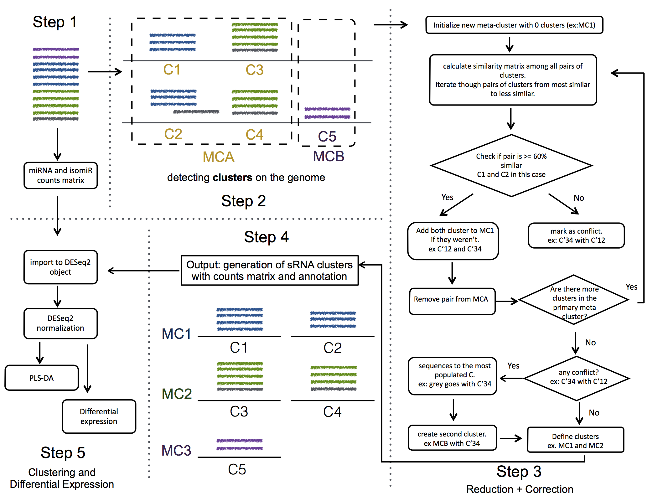
Small RNA clusters
We use seqcluster to identify any type of small RNA. It generates a list of clusters of small RNA sequences, their genome location, their annotation and the abundance in all the sample of the project. The next figure explain the algorithm used for that and the way to use it for differential expression analyses.
{ width=50% }
This file generated by seqcluster, seqcluster.db, can be used with the page reader.html after downloading from here.
See example:
SmallRNA types detected
metadata(experiments(bcb)[["cluster"]])[["size"]] %>%
    ggplot(aes(x = size, y = pct, fill = priority)) +
    geom_bar(stat = "identity", position = "dodge")
bcbSmallCluster(bcb)
Clustering of samples
data = bcbSmallPCA(bcb, "cluster")
color_by = metadata(bcb)[["interesting_groups"]]
palette <- colorRamp2(seq(min(data[["counts"]]),
                          max(data[["counts"]]), length = 3),
                      c("blue", "#EEEEEE", "orange"), space = "RGB")
th <- HeatmapAnnotation(df = data[["annotation"]],
                        col = degColors(data[["annotation"]]))
Heatmap(data[["counts"]],
        col = palette,
        top_annotation = th,
        clustering_method_rows = "ward.D",
        clustering_distance_columns = "kendall",
        clustering_method_columns = "ward.D",
        show_row_names = FALSE,
        show_column_names = ncol(data[["counts"]]) < 50)
degPCA(data[["counts"]], data[["annotation"]],
            condition = color_by)
Session
devtools::session_info()
lpantano/bcbioSmallRna documentation built on March 5, 2020, 9:17 a.m.
R Package Documentation
Browse R Packages
We want your feedback!
Note that we can't provide technical support on individual packages. You should contact the package authors for that.
library(BiocStyle) knitr::opts_chunk$set(tidy=FALSE, dev="png", message=FALSE, error=FALSE, warning=TRUE) library(knitr) library(ggplot2) # Set seed for reproducibility set.seed(1454944673L) theme_set( theme_light(base_size = 11L)) theme_update( legend.justification = "center", legend.position = "bottom")
library(isomiRs) library(DEGreport) library(bcbioSmallRna) library(ComplexHeatmap) library(circlize) data(sbcb) # bcbioSmallRnaDataSet bcb <- sbcb
Exploratory analysis
In this section we will see descriptive figures about quality of the data, reads with adapter, reads mapped to miRNAs, reads mapped to other small RNAs.
Size distribution
After adapter removal, we can plot the size distribution of the small RNAs. We expect the majority of reads to have adapters and we expect a peak at 22 (maybe 33 as well) that indicates miRNA/tRNA enrichment. There are some cases this rule won't apply.
bcbSmallSize(bcb)
bcbSmallSizeDist(bcb)
miRNA
A microRNA (abbreviated miRNA) is a small non-coding RNA molecule (containing about 22 nucleotides) found in plants, animals and some viruses, that functions in RNA silencing and post-transcriptional regulation of gene expression.[https://en.wikipedia.org/wiki/MicroRNA]
Total miRNA expression annotated with mirbase
miRBase is one of the database that contains the reference miRNA sequences. We used this database to annotate the sequences with miraligner
bcbSmallMicro(bcb)
Clustering of samples
data = bcbSmallPCA(bcb) color_by = metadata(bcb)[["interesting_groups"]]
palette <- colorRamp2(seq(min(data[["counts"]]), max(data[["counts"]]), length = 3), c("blue", "#EEEEEE", "orange"), space = "RGB") th <- HeatmapAnnotation(df = data[["annotation"]], col = degColors(data[["annotation"]])) Heatmap(data[["counts"]], col = palette, top_annotation = th, clustering_method_rows = "ward.D", clustering_distance_columns = "kendall", clustering_method_columns = "ward.D", show_row_names = FALSE, show_column_names = ncol(data[["counts"]]) < 50)
degPCA(data[["counts"]], data[["annotation"]], condition = color_by)
isomiRs
isomiR is a term coined by Morin et al. to refer to those sequences that have variations with respect to the reference MiRNA sequence. [https://en.wikipedia.org/wiki/IsomiR]
There are 5 different types of isomiRs:
- ref: perfect match to the sequence on the database
- t3: nucleotides changes at 3'
- t5: nucleotides changes at 5'
- add: nucleotides addition at the 3'
- mism: putatives SNPs
ids <- bcbio(bcb, "isomirs") isoPlot(ids, type = "all", column = color_by)
Small RNA clusters
We use seqcluster to identify any type of small RNA. It generates a list of clusters of small RNA sequences, their genome location, their annotation and the abundance in all the sample of the project. The next figure explain the algorithm used for that and the way to use it for differential expression analyses.
{ width=50% }
This file generated by seqcluster, seqcluster.db, can be used with the page reader.html after downloading from here.
See example:
SmallRNA types detected
metadata(experiments(bcb)[["cluster"]])[["size"]] %>% ggplot(aes(x = size, y = pct, fill = priority)) + geom_bar(stat = "identity", position = "dodge")
bcbSmallCluster(bcb)
Clustering of samples
data = bcbSmallPCA(bcb, "cluster") color_by = metadata(bcb)[["interesting_groups"]]
palette <- colorRamp2(seq(min(data[["counts"]]), max(data[["counts"]]), length = 3), c("blue", "#EEEEEE", "orange"), space = "RGB") th <- HeatmapAnnotation(df = data[["annotation"]], col = degColors(data[["annotation"]])) Heatmap(data[["counts"]], col = palette, top_annotation = th, clustering_method_rows = "ward.D", clustering_distance_columns = "kendall", clustering_method_columns = "ward.D", show_row_names = FALSE, show_column_names = ncol(data[["counts"]]) < 50)
degPCA(data[["counts"]], data[["annotation"]], condition = color_by)
Session
devtools::session_info()
R Package Documentation
Browse R Packages
We want your feedback!
Note that we can't provide technical support on individual packages. You should contact the package authors for that.
Embedding an R snippet on your website
Add the following code to your website.
For more information on customizing the embed code, read Embedding Snippets.